Part 2.1
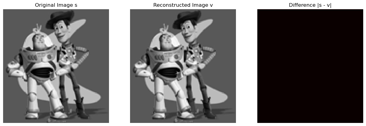
This code implements Poisson image reconstruction, a computational method used to reconstruct a grayscale image from its gradients. The reconstruction is governed by mathematical constraints on the horizontal and vertical gradients of the image, ensuring that the gradients of the reconstructed image closely match those of the input. Additionally, a fixed point constraint is applied to remove ambiguity caused by the unknown constant offset in gradient-based reconstruction.
In mathematical terms, let \( s(x,y) \) represent the input grayscale image. The reconstruction is based on the following principles:
-
Gradient Constraints:
-
Horizontal gradients: \( s(x+1,y) - s(x,y) = v(x+1,y) - v(x,y) \)
-
Vertical gradients: \( s(x,y+1) - s(x,y) = v(x,y+1) - v(x,y) \)
These equations ensure that the reconstructed image \( v(x,y) \) retains the gradient characteristics of the input \( s(x,y) \).
-
Fixed Point Constraint:
-
One pixel value is fixed to resolve the constant ambiguity: \( v(0,0) = s(0,0) \)
The above constraints are assembled into a sparse linear system of equations, represented as:
\[
A \cdot \mathbf{v} = \mathbf{b}
\]
Where:
- \( A \) is a sparse matrix encoding the gradient constraints,
- \( \mathbf{b} \) contains the gradient differences from \( s(x,y) \),
- \( \mathbf{v} \) represents the unknown pixel values of the reconstructed image.
The least-squares solution to this system is:
\[
\mathbf{v} = \text{argmin}_{\mathbf{v}} \| A \cdot \mathbf{v} - \mathbf{b} \|^2
\]
This problem is efficiently solved using the `scipy.sparse.linalg.lsqr` function.
After solving, the pixel values \( \mathbf{v} \) are reshaped to the image dimensions and clipped to the valid range [0,255]. The code then computes the mean squared error (MSE) to evaluate the reconstruction quality, defined as:
\[
\text{MSE} = \frac{1}{N} \sum_{x, y} \left( s(x, y) - v(x, y) \right)^2
\]
where \( N \) is the total number of pixels.
The main function orchestrates the process by:
- Loading the input image \( s(x,y) \),
- Performing the reconstruction using `poisson_reconstruct`,
- Calculating and printing the MSE,
- Visualizing the original image, reconstructed image, and the absolute difference between them.
Part 2.2
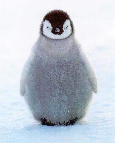
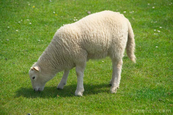
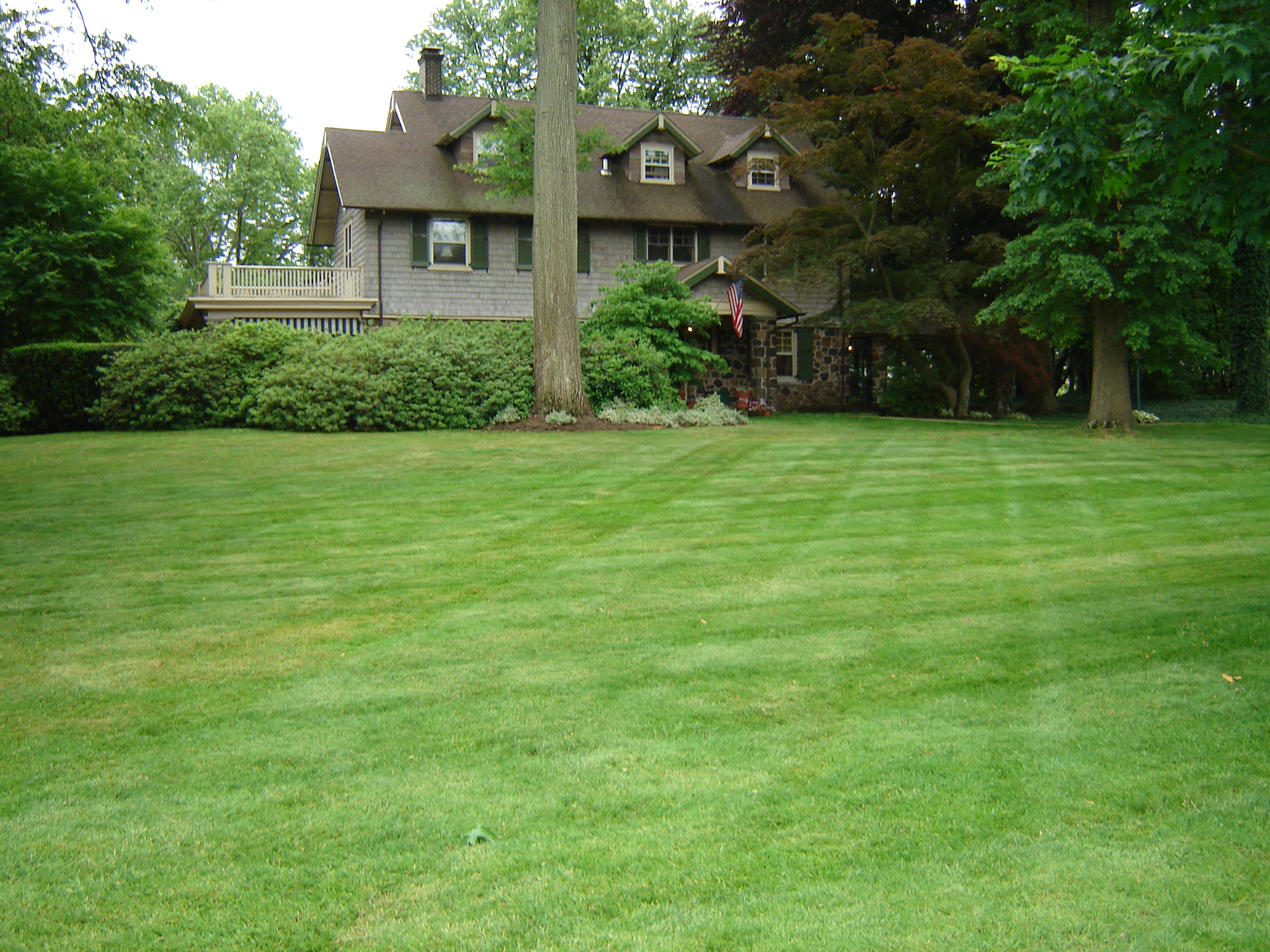
I developed this code to implement Poisson Image Blending, a technique that allows for seamless integration of a source object into a target background while ensuring smooth gradient transitions at the boundaries. The process begins with interactive region selection, where I use the `getMask` function to let the user draw a polygon around the desired object in the source image. This polygon is converted into a binary mask \( \text{Mask}(x,y) \), defined as:
\[
\text{Mask}(x, y) = \begin{cases}
1, & \text{if } (x, y) \text{ is inside the polygon}, \\
0, & \text{otherwise}.
\end{cases}
\]
The precision of the mask depends on the image resolution and the complexity of the polygon defined by the vertices \( (x_i, y_i) \). The result is a binary matrix representing the selected region and a list of the polygon's vertices for further processing.
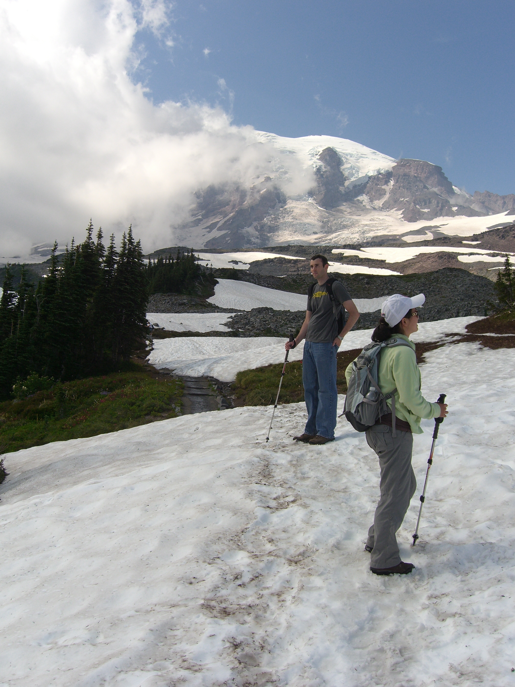
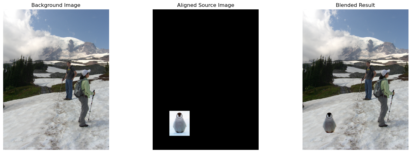
Next, I align the source image and mask to the target image using the `alignSource` function. The user selects a point in the target image to specify where the source object should be placed. To facilitate accurate placement, I calculate a scale factor:
\[
\text{Scale Factor} = \frac{\text{Original Dimension}}{\text{Resized Dimension}}.
\]
This scales the target image for better viewing during selection. The source image is then aligned by calculating the bounding box:
\[
\begin{align*}
\text{Top Left} &= \left( x_t - \frac{W_s}{2},\ y_t - \frac{H_s}{2} \right), \\
\text{Bottom Right} &= \left( x_t + \frac{W_s}{2},\ y_t + \frac{H_s}{2} \right),
\end{align*}
\]
where \( x_t, y_t \) are the coordinates of the selected target point, and \( W_s, H_s \) are the width and height of the source image. This alignment ensures that the source object fits within the bounds of the target image.
The core of the blending process involves solving the Poisson equation, implemented in the `poisson_reconstruct` function. The goal is to reconstruct the selected region in the target image by ensuring gradient continuity between the source and the surrounding target area. For each pixel \( (x,y) \) inside the mask, I apply the discrete Laplacian operator:
\[
\Delta v(x, y) = 4v(x, y) - v(x+1, y) - v(x-1, y) - v(x, y+1) - v(x, y-1),
\]
and set up the equation:
\[
\Delta v(x, y) = \Delta s(x, y),
\]
where \( v(x, y) \) is the pixel value in the blended image, and \( s(x, y) \) is the pixel value in the source image. This ensures that the gradient (Laplacian) of the blended image matches that of the source image within the mask. For pixels on the boundary, I incorporate the target image's pixel values to maintain consistency:
\[
v(x, y) = t(x, y), \quad \text{for } (x, y) \notin \text{Mask},
\]
where \( t(x, y) \) is the pixel value in the target image. I construct a sparse linear system \( A \mathbf{v} = \mathbf{b} \), where:
- \( A \) is a sparse matrix encoding the relationships defined by the Laplacian operator.
- \( \mathbf{v} \) is the vector of unknown pixel values within the mask.
- \( \mathbf{b} \) is a vector incorporating the source image gradients and boundary conditions.
Specifically, for each variable pixel \( v_i \):
- \( A[i,i] = 4 \),
- and for each neighbor \( v_j \) connected to \( v_i \): \( A[i,j] = -1 \).
The right-hand side vector \( \mathbf{b} \) is calculated based on the gradients from the source image and the known pixel values from the target image at the boundary. I solve this system using a sparse linear solver, minimizing the equation:
\[
\| A \cdot \mathbf{v} - \mathbf{b} \|^2.
\]
This yields the pixel values \( \mathbf{v} \) that seamlessly blend the source object into the target background.
In the `poisson_blend` function, I apply this blending process independently to each color channel (Red, Green, Blue) to preserve the color integrity of the image. For each channel \( c \), the blending ensures:
\[
v_c(x, y) = \begin{cases}
t_c(x, y), & \text{if } (x, y) \notin \text{Mask}, \\
\text{Solution from Poisson Equation}, & \text{if } (x, y) \in \text{Mask},
\end{cases}
\]
where \( v_c(x, y) \) is the blended pixel value for channel \( c \), and \( t_c(x, y) \) is the target pixel value for channel \( c \).
Finally, in the main function, I bring all these steps together. The user selects the source region and its placement in the target image. The source is then aligned and blended into the target using the Poisson blending technique.
This code provides a robust framework for Poisson image blending, combining interactive tools
Bells and whistle——Color2Gray
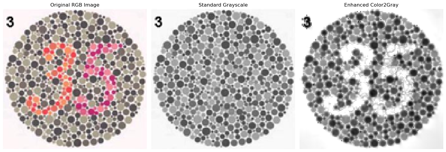
This code provides an advanced implementation of color-to-grayscale conversion, improving upon the traditional grayscale methods by preserving perceptually important gradients and visual contrasts. The approach blends information from the RGB color space and the HSV (hue, saturation, value) color space to generate a grayscale image that better reflects the visual characteristics of the original colored image.
The process starts with the `get_hsv_gradients` function, which extracts the gradients of the saturation and value channels from the HSV color representation. The RGB image is first converted to HSV, where the saturation (S) and value (V) channels are processed to compute their gradients:
\[
\begin{aligned}
S_{gx} &= \frac{\partial S}{\partial x}, \quad S_{gy} = \frac{\partial S}{\partial y}, \\
V_{gx} &= \frac{\partial V}{\partial x}, \quad V_{gy} = \frac{\partial V}{\partial y}.
\end{aligned}
\]
The gradient magnitudes for these channels are calculated as:
\[
S_{\text{grad mag}} = \sqrt{S_{gx}^2 + S_{gy}^2}, \quad V_{\text{grad mag}} = \sqrt{V_{gx}^2 + V_{gy}^2}.
\]
A weighting parameter \( \alpha \) combines the saturation and value gradients into weighted gradients:
\[
\text{Weights} = \frac{\alpha \cdot S \cdot S_{\text{grad mag}}}{V_{\text{grad mag}} + \epsilon},
\]
where \( \epsilon \) prevents division by zero. These weighted gradients combine the saturation and value gradients into final gradients for use in grayscale reconstruction:
\[
G_x = \text{Weights} \cdot S_{gx} + V_{gx}, \quad G_y = \text{Weights} \cdot S_{gy} + V_{gy}.
\]
The `color2gray` function combines these gradients with a traditional grayscale version of the image to enforce consistency in intensity and gradient magnitudes. It formulates the problem as a linear system, balancing two objectives: gradient consistency and intensity matching.
To model gradient consistency, the gradients are incorporated into a sparse matrix \( A \), encoding the relationships between neighboring pixels. For each horizontal and vertical neighbor, the matrix \( A \) and vector \( \mathbf{b} \) are updated with gradient-weighted equations:
\[
A[i,j] = \begin{cases}
-\text{Gradient Weight}, & \text{if } j \text{ is a neighbor of } i, \\
+\text{Gradient Weight}, & \text{if } j = i,
\end{cases} \quad \mathbf{b}[i] = \text{Gradient Weight} \cdot G_x \text{ or } G_y.
\]
For intensity matching, an additional set of equations ensures that the grayscale intensities align with the standard grayscale version, weighted by a parameter \( \lambda \):
\[
A[i, i] = \lambda \cdot \left( 1 + \text{Gray Gradient Magnitude} \right), \quad \mathbf{b}[i] = \lambda \cdot \text{Standard Gray}[i].
\]
The combined system is solved using a sparse linear solver, minimizing:
\[
\| A \cdot \mathbf{v} - \mathbf{b} \|^2,
\]
where \( \mathbf{v} \) is the vector of unknown grayscale intensities.
The resulting grayscale image is post-processed to adjust its dynamic range. A histogram matching function aligns the intensity levels of the enhanced grayscale image with the standard grayscale image to maintain visual consistency. For each intensity level:
\[
\text{Adjusted Intensity} = \text{Source Intensity} \cdot \frac{\text{Mean Target Intensity}}{\text{Mean Source Intensity} + \epsilon}.
\]
The `process_image` function brings these steps together. It loads an RGB image, computes both the standard and enhanced grayscale versions, and visualizes the results. The enhanced grayscale image retains critical visual details from the color image by leveraging gradients in the HSV space, ensuring that the perceptual importance of color information is preserved in the grayscale conversion.
