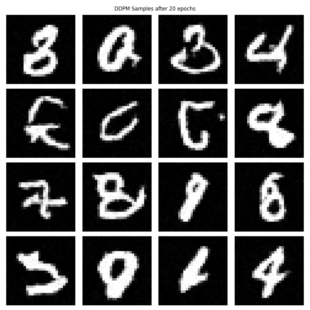
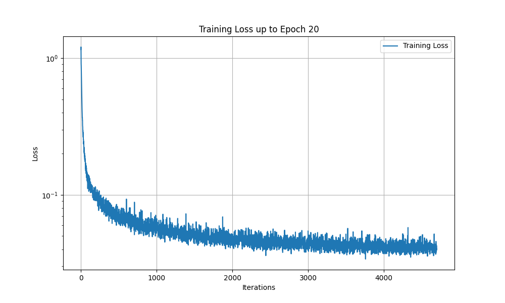
Part 2.1
Part 2.1: Time Conditioning to UNet
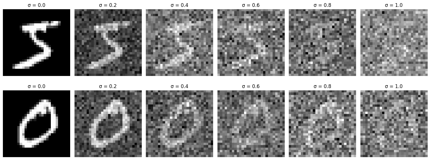
In implementing the diffusion model, I delved deeply into the mathematical foundations of stochastic processes and denoising score matching. The core idea revolves around modeling the data distribution by progressively adding Gaussian noise and then training a model to reverse this process. This approach allows the model to generate new data samples that closely resemble the original data distribution.
Forward Diffusion Process
The forward diffusion process incrementally adds Gaussian noise to the data over \( T \) timesteps. At each timestep \( t \), noise is added according to a predefined schedule. Mathematically, this process is defined as:
\[
q(\mathbf{x}_t \mid \mathbf{x}_{t-1}) = \mathcal{N}\left( \mathbf{x}_t; \sqrt{\alpha_t} \mathbf{x}_{t-1}, \beta_t \mathbf{I} \right),
\]
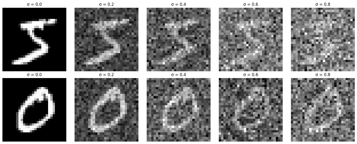
where \( \alpha_t = 1 - \beta_t \) and \( \beta_t \) is the noise variance at timestep \( t \). By composing these transitions, the noisy data at any timestep \( t \) can be expressed directly in terms of the original data \( \mathbf{x}_0 \):
\[
\mathbf{x}_t = \sqrt{\bar{\alpha}_t} \mathbf{x}_0 + \sqrt{1 - \bar{\alpha}_t} \boldsymbol{\epsilon},
\]
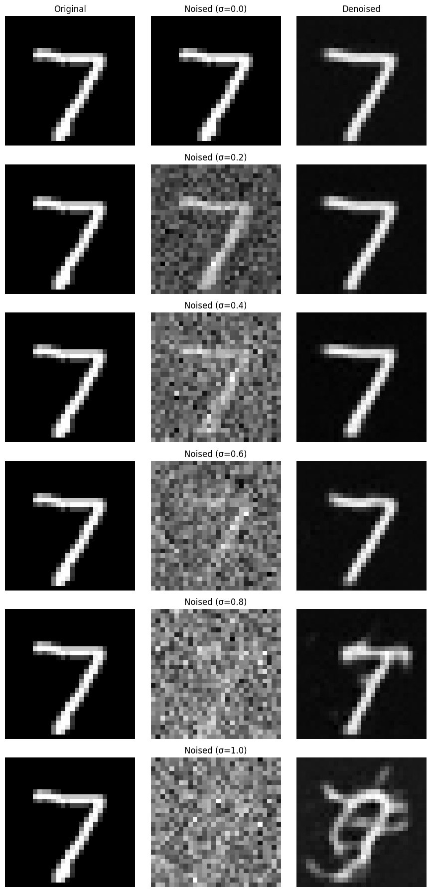
with \( \bar{\alpha}_t = \prod_{s=1}^t \alpha_s \) and \( \boldsymbol{\epsilon} \sim \mathcal{N}(\mathbf{0}, \mathbf{I}) \). This equation shows that the data becomes increasingly noisy as \( t \) increases.
Noise Schedule
The noise schedule determines how \( \beta_t \) changes over time. A linear schedule interpolating between a starting value \( \beta_{\text{start}} \) and an ending value \( \beta_{\text{end}} \) is used:
\[
\beta_t = \beta_{\text{start}} + \frac{t}{T} \left( \beta_{\text{end}} - \beta_{\text{start}} \right).
\]
This schedule affects the cumulative product \( \bar{\alpha}_t \), which is crucial for both the forward diffusion and reverse denoising processes.
Reverse Diffusion Process
The goal is to learn the reverse of the forward process, denoted as \( p_\theta(\mathbf{x}_{t-1} \mid \mathbf{x}_t) \), which ideally inverts the noise addition:
\[
p_\theta(\mathbf{x}_{t-1} \mid \mathbf{x}_t) = \mathcal{N}\left( \mathbf{x}_{t-1}; \boldsymbol{\mu}_\theta(\mathbf{x}_t, t), \sigma_t^2 \mathbf{I} \right).
\]
Here, \( \boldsymbol{\mu}_\theta \) is the mean predicted by a neural network conditioned on \( \mathbf{x}_t \) and \( t \), and \( \sigma_t^2 \) is the variance, which can be set based on the forward process.
Training Objective
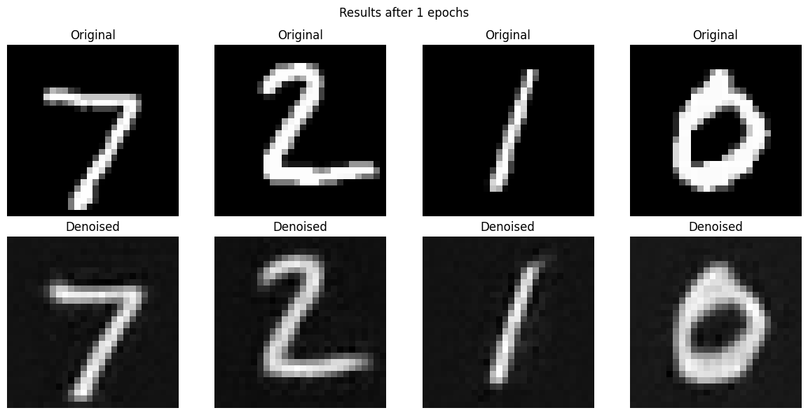
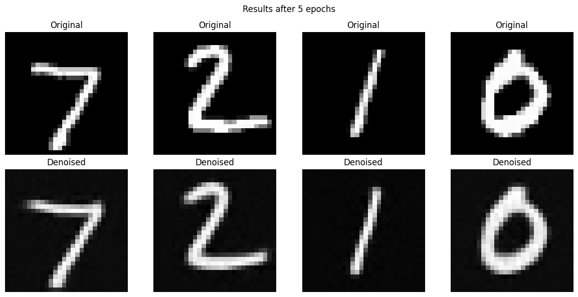
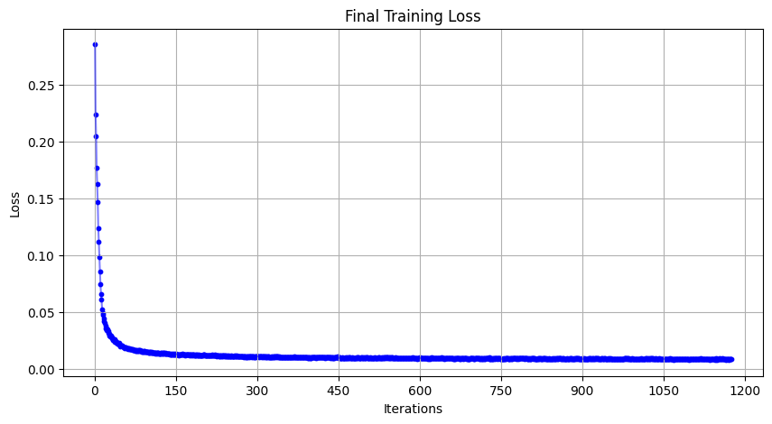
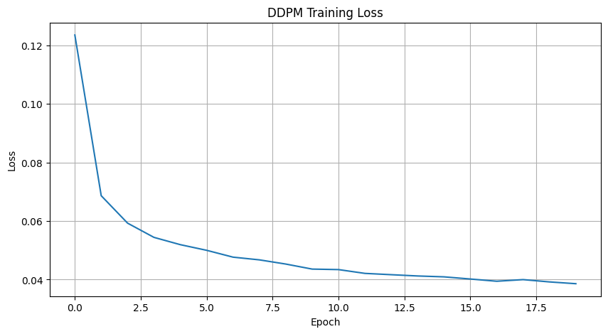
Training aims to minimize the difference between the true noise \( \boldsymbol{\epsilon} \) and the noise predicted by the neural network \( \boldsymbol{\epsilon}_\theta \). The simplified loss function used is:
\[
\mathcal{L} = \mathbb{E}_{\mathbf{x}_0, \boldsymbol{\epsilon}, t} \left[ \left\| \boldsymbol{\epsilon} - \boldsymbol{\epsilon}_\theta(\mathbf{x}_t, t) \right\|^2 \right].
\]
This loss is derived from variational lower bounds and is a form of denoising score matching, encouraging the model to accurately predict the noise at each timestep.
Time-Conditioned Neural Network
The neural network \( \boldsymbol{\epsilon}_\theta \) is designed to predict the noise present in the data at each timestep. It is conditioned on \( t \) to account for the time-dependent nature of the noise addition. The network architecture includes:
- Time Embedding: Encoding the timestep \( t \) into a higher-dimensional representation to provide temporal information to the network.
- UNet Architecture: A convolutional network with downsampling and upsampling paths, capturing multi-scale spatial features and allowing skip connections for efficient gradient flow.
Sampling Procedure
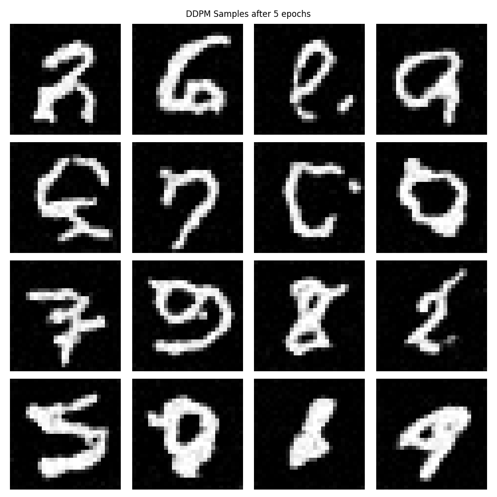
To generate new samples, the process starts with Gaussian noise \( \mathbf{x}_T \) and iteratively applies the learned reverse transitions:
\[
\mathbf{x}_{t-1} = \frac{1}{\sqrt{\alpha_t}} \left( \mathbf{x}_t - \frac{\beta_t}{\sqrt{1 - \bar{\alpha}_t}} \boldsymbol{\epsilon}_\theta(\mathbf{x}_t, t) \right) + \sigma_t \mathbf{z},
\]
where \( \mathbf{z} \sim \mathcal{N}(\mathbf{0}, \mathbf{I}) \) if \( t > 1 \) and \( \mathbf{z} = \mathbf{0} \) if \( t = 1 \), and \( \sigma_t = \sqrt{\beta_t} \). This equation updates the sample by removing the estimated noise and adding a small amount of random noise to maintain stochasticity, gradually refining the sample towards the data distribution.
Mathematical Derivation of Key Terms
- Cumulative Product of Alphas:
\[
\bar{\alpha}_t = \prod_{s=1}^t \alpha_s.
\]
- Variance Terms:
\[
\beta_t = 1 - \alpha_t,
\]
\[
\tilde{\beta}_t = \beta_t \frac{1 - \bar{\alpha}_{t-1}}{1 - \bar{\alpha}_t}.
\]
- Mean of Reverse Process:
The mean \( \boldsymbol{\mu}_\theta(\mathbf{x}_t, t) \) for the reverse process is derived based on the posterior distribution \( q(\mathbf{x}_{t-1} \mid \mathbf{x}_t, \mathbf{x}_0) \):
\[
\boldsymbol{\mu}_\theta(\mathbf{x}_t, t) = \frac{1}{\sqrt{\alpha_t}} \left( \mathbf{x}_t - \frac{\beta_t}{\sqrt{1 - \bar{\alpha}_t}} \boldsymbol{\epsilon}_\theta(\mathbf{x}_t, t) \right).
\]
Theoretical Foundations
This approach is grounded in several theoretical concepts:
- Stochastic Differential Equations (SDEs): The diffusion process can be viewed as a discretization of an SDE, connecting discrete timesteps to continuous-time diffusion models.
- Score Matching: The model implicitly estimates the score function \( \nabla_{\mathbf{x}} \log q_t(\mathbf{x}) \), which is the gradient of the log probability density of the noisy data at timestep \( t \).
- Variational Inference: The training objective is derived from maximizing a variational lower bound on the data likelihood, framing the diffusion model within probabilistic modeling and allowing for principled training.
Practical Implementation Details
- Random Timestep Selection: During training, timesteps \( t \) are randomly sampled for each data point to ensure the model learns to denoise across all stages of the diffusion process.
- Normalization of Timestep: The timestep \( t \) is normalized (e.g., \( t / T \)) before being input into the network, which helps in stabilizing training and improving performance.
- Loss Computation: The mean squared error loss between the true noise \( \boldsymbol{\epsilon} \) and the predicted noise \( \boldsymbol{\epsilon}_\theta(\mathbf{x}_t, t) \) guides the model to accurately estimate the noise component at each timestep.
Conclusion
By integrating these mathematical concepts, the model effectively learns to reverse the diffusion process, transforming noisy data back into samples from the original data distribution. The time-conditioned neural network captures both the temporal dynamics of noise addition and the spatial structures within the data, allowing for accurate noise prediction and high-quality sample generation. This method leverages the interplay between stochastic processes, neural network approximation, and probabilistic modeling to model complex data distributions and generate new, realistic data samples.
guidance_scale=5
Part 2.2
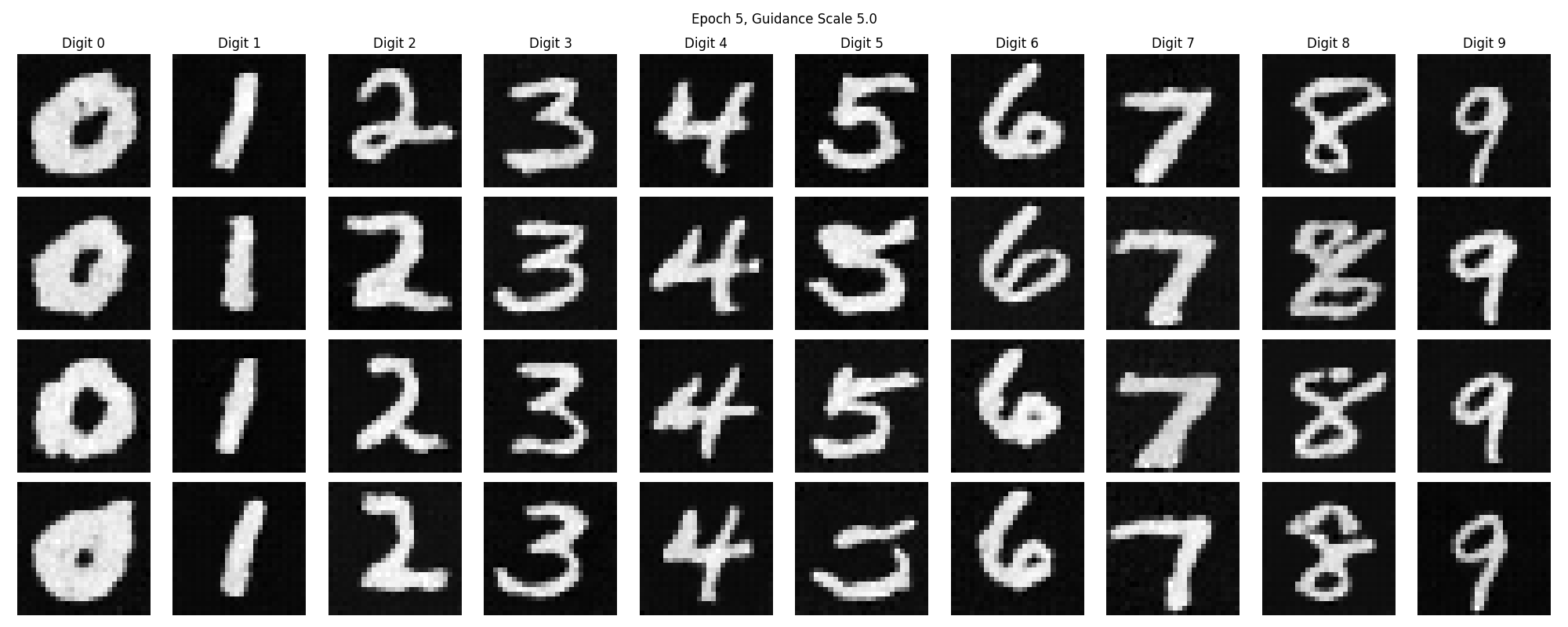
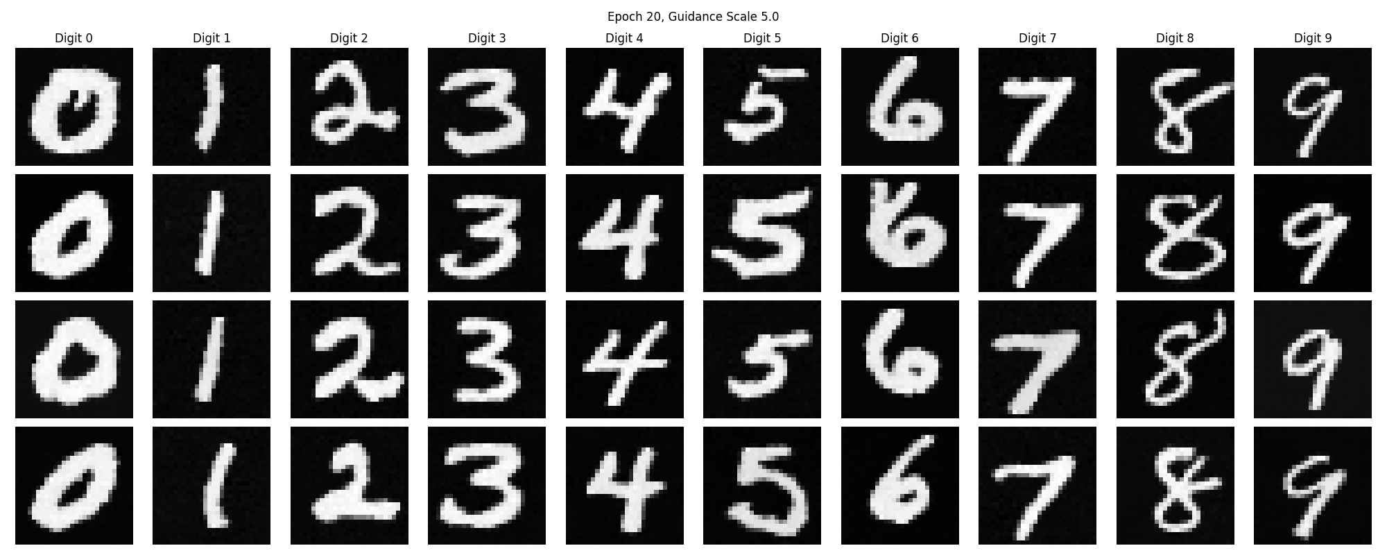
Part 2.2: Class Conditioning to UNet
In extending the diffusion model, I focused on implementing a class-conditioned UNet to incorporate label information into the generative process. This enhancement allows the model not only to generate data that resembles the training distribution but also to control the specific class of the generated samples. The mathematical foundations remain rooted in diffusion processes and denoising score matching, with additional mechanisms to handle class conditioning.
To incorporate class information, I modified the neural network \( \boldsymbol{\epsilon}_\theta \) to accept the class label \( c \) alongside the noisy input \( \mathbf{x}_t \) and the timestep \( t \):
\[
\boldsymbol{\epsilon}_\theta(\mathbf{x}_t, c, t).
\]
This modification enables the model to generate class-specific denoising predictions. The architecture includes input convolutional layers to process the noisy input, downsampling blocks to reduce spatial dimensions while increasing feature richness, and flattening layers to transition between convolutional and fully connected layers. Time and class embeddings are generated using fully connected layers that transform \( t \) and \( c \) into embeddings \( t_1, t_2 \) and \( c_1, c_2 \). These embeddings are integrated into the network at specific points, scaling and shifting the feature maps via element-wise operations. Skip connections are used to concatenate feature maps from downsampling layers with upsampling layers, enriched with class and time information.
The forward diffusion process remains similar, where the noisy input \( \mathbf{x}_t \) is generated as:
\[
\mathbf{x}_t = \sqrt{\bar{\alpha}_t} \mathbf{x}_0 + \sqrt{1 - \bar{\alpha}_t} \boldsymbol{\epsilon},
\]
with \( \mathbf{x}_0 \) being the original data sample and \( \boldsymbol{\epsilon} \sim \mathcal{N}(\mathbf{0}, \mathbf{I}) \) representing Gaussian noise. The noise schedule is defined with betas \( \beta_t \) linearly spaced between \( \beta_{\text{start}} \) and \( \beta_{\text{end}} \), and alphas \( \alpha_t = 1 - \beta_t \), determining the amount of signal retained at each timestep.
The training objective is adjusted to include class conditioning. The loss function aims to minimize:
\[
\mathcal{L} = \mathbb{E}_{\mathbf{x}_0, c, \boldsymbol{\epsilon}, t} \left[ \left\| \boldsymbol{\epsilon} - \boldsymbol{\epsilon}_\theta(\mathbf{x}_t, c, t) \right\|^2 \right],
\]
where the expectation is over data samples \( \mathbf{x}_0 \), class labels \( c \), noise \( \boldsymbol{\epsilon} \), and timesteps \( t \). The goal is to train the network to predict the added noise conditioned on both \( \mathbf{x}_t \) and \( c \).
To enhance sample quality and adherence to the desired class, I implemented classifier-free guidance. This mechanism allows adjusting the influence of class conditioning during sampling. During training, with probability \( p_{\text{uncond}} \), the class label is omitted, effectively training the model to handle both conditional and unconditional cases. The guided prediction during sampling is computed as:
\[
\boldsymbol{\epsilon}_{\text{guided}} = \boldsymbol{\epsilon}_{\text{uncond}} + s \left( \boldsymbol{\epsilon}_{\text{cond}} - \boldsymbol{\epsilon}_{\text{uncond}} \right),
\]
where \( s \) is the guidance scale controlling the strength of conditioning.
The sampling procedure with class conditioning involves iterative reverse diffusion, starting from \( \mathbf{x}_T \sim \mathcal{N}(\mathbf{0}, \mathbf{I}) \). At each timestep \( t \), conditional and unconditional predictions are computed, and classifier-free guidance is applied to update the sample:
\[
\mathbf{x}_{t-1} = \frac{1}{\sqrt{\alpha_t}} \left( \mathbf{x}_t - \frac{\beta_t}{\sqrt{1 - \bar{\alpha}_t}} \boldsymbol{\epsilon}_{\text{guided}} \right) + \sigma_t \mathbf{z},
\]
where \( \sigma_t = \sqrt{\beta_t} \) and \( \mathbf{z} \sim \mathcal{N}(\mathbf{0}, \mathbf{I}) \) if \( t > 1 \), else \( \mathbf{0} \). This equation updates the sample by removing the estimated guided noise and adding a small amount of random noise to maintain stochasticity.
To implement classifier-free guidance during training, I introduced a mask \( m \) where \( m = 1 \) with probability \( 1 - p_{\text{uncond}} \) (using the class label) and \( m = 0 \) with probability \( p_{\text{uncond}} \) (dropping the class label). The modified class input becomes:
\[
c_{\text{input}} = m \cdot c_{\text{one-hot}},
\]
where \( c_{\text{one-hot}} \) is the one-hot encoding of the class label. The loss function remains the mean squared error between the true noise and the predicted noise.
This approach has several advantages. It allows controlled generation, enabling the model to generate specific classes on demand. The guidance can enhance fidelity to class characteristics, improving sample quality. Additionally, the adjustable guidance scale \( s \) provides flexibility in balancing diversity and accuracy in the generated samples.
By integrating class conditioning into the diffusion model, the neural network learns to incorporate label information into the denoising process. The mathematical framework extends the original diffusion model to handle additional conditioning variables, while classifier-free guidance provides a powerful tool to control the influence of conditioning during sampling. This approach combines the strengths of diffusion models in capturing complex data distributions with the ability to generate class-specific samples, enhancing both the versatility and utility of the generative model.
guidance_scale=5
